10 Python Tips for High-Performance ML Backends (1)

This article is a translated version of my article posted on Hyperconnect Tech Blog, originally written in Korean at May 2023.
한국어 포스트를 보시려면 위 링크를 클릭해주세요.

Article by Youngsoo Lee (me), Suhyun Lee, and Gunjun Lee. Hyperconnect, May 2023.

Python is a great language that’s easy to learn and has a strong open-source ecosystem, especially for ML libraries. Because it’s so convenient, many companies use Python not only for data analysis and model training, but also for backend servers. (For example, Instagram uses Python in its backend servers [0-1].) At Hyperconnect, many of our ML backend servers are also written in Python. However, one big downside of Python is that it’s slow to run. While Python is great for ML, running it in backend servers where response time matters has caused a lot of pain due to this slow speed.

Even if Python is slow, switching to a faster language like C++, Go, Rust, or Kotlin is not easy. Rewriting the whole business logic takes a lot of time, and it’s also hard to give up the benefits of libraries like Numpy and PyTorch. We’ve also faced many situations where switching languages wasn’t practical, and through that, we’ve discovered several tricks to make Python run faster and meet performance requirements.

In this post, we’ll share 10 performance optimization tips we’ve learned while running various Python-based ML backend servers at Hyperconnect. These tips are especially useful for ML workloads that deal with large amounts of data. We’ll also cover how to use popular third-party libraries more effectively. We won’t talk about solutions like Pypy, Numba, or C bindings here, since they can be hard to maintain and may cause pushback from the team. Some of these tips can reduce server response time by more than half with just a few lines of code, so we hope you enjoy the read.

Note: Since most people use the CPython implementation of Python [0-2], this post is also written with CPython in mind.

Part 1 (current)
1. GC can be a bottleneck in some cases. You can tune when GC runs.
2. Built-in lists aren’t always fast — use array or numpy when needed
3. Multiprocessing has high communication overhead — be careful in low-latency scenarios
4. If you’re using PyTorch in a multiprocess environment, adjust num_threads
5. Pydantic is very slow — avoid it when not needed

Part 2
6. Creating a Pandas DataFrame is slow. Use it carefully.
7. The default json package is slow. Use orjson or ujson.
8. Classes are not always fast. Use dict if performance is an issue.
9. Python 3.11 is less slow
10. (Bonus) How to use line profiler

#1 GC can be a bottleneck in some cases. You can tune when GC runs.

In most backend servers written in Python, it’s rare to create hundreds of objects per request. So garbage collection (GC) usually doesn’t cause major latency issues. But in ML backends that handle large data, it’s different. For example, a recommendation API server might create thousands or tens of thousands of objects for each request. In such cases, GC can become a problem. At Hyperconnect, we’ve seen our recommendation APIs slow down due to GC, and by tweaking just a few lines of code to adjust GC settings, we were able to cut the P99 latency to one-third.

So how and why does GC cause problems? To explain that, let’s briefly look at how Python’s garbage collection works.

Python GC

In Python, objects that are no longer used are usually cleaned up through reference counting. Each object tracks how many references point to it, and when that count drops to zero, the object is deleted [1-1, 1-2]. But reference counting has limits. If two or more objects refer to each other in a cycle, they can’t be deleted even when they are no longer needed (like a circular linked list). So Python also runs a separate process called cyclic garbage collection to handle these cases. (By the way, Java and other JVM languages use tracing garbage collection [1-3] instead.)

Reference counting is usually very fast. The performance problem comes from cyclic GC. To remove these “garbage” objects, Python first has to find them. How? It builds a reference graph of all objects in memory and looks for unreachable cycles. Since this involves scanning all memory, it can be slow.

To make this faster, Python uses a trick called “Generational GC”, which is similar to the weak generational hypothesis used in the JVM [1-4]. The idea is that most objects die young, and old objects are usually still in use (like global variables). So instead of scanning everything every time, Python only scans objects in certain generations more often than others.

Python Generation GC

So how are these generations managed in Python, and how often does GC run for each one?

In Python, objects belong to generation 0, 1, or 2 depending on how many GC cycles they’ve survived. New objects start in gen 0. If they survive one GC, they move to gen1, and then to gen2 after another survival. Python controls how often each generation is collected using thresholds, which you can check with gc.get_threshold().

>>> import gc
>>> gc.get_threshold()
(700, 10, 10)

These numbers mean:

Gen 0 GC runs when the number of new allocations minus deallocations exceeds 700.
Gen 1 GC runs after 10 Gen 0 GCs.
Gen 2 GC runs after 10 Gen 1 GCs, and only if an extra condition is also met (to avoid slowing down performance too much) [1-5].

GC Overhead

In ML backend servers that create many objects per request, cyclic GC can run often and slow things down.

Here’s a simple example. We create many dummy objects and measure the average and max creation times. We also import PyTorch and Numpy (not used directly) to increase memory usage.

import time

import numpy as np
import torch

class DummyClass:
    def __init__(self):
        self.foo = [[] for _ in range(4)]

def generate_objects() -> None:
    bar = [DummyClass() for _ in range(1000)]

times = []
for _ in range(500):
    start_time = time.time()
    generate_objects()
    times.append(time.time() - start_time)

avg_elapsed_time = sum(times) / len(times) * 1000
max_elapsed_time = max(times) * 1000

print(f"avg time: {avg_elapsed_time:.2f}ms, max time: {max_elapsed_time:.2f}ms")

Results:

avg time: 2.08ms, max time: 22.45ms

There’s a big difference between the average and the worst case. But is this because of GC? Let’s test again with GC turned off using gc.disable():

import gc
...
gc.disable()
...

Results:

avg time: 0.73ms, max time: 0.88ms

Now the max time is much lower — 25 times faster than before. This kind of latency spike can seriously affect P99 latency in production servers.

You can also try turning off only Gen 2 GC with gc.set_threshold(700, 0, 99999999). In that case, results were:

avg time: 0.91ms, max time: 1.15ms

Still slower than disabling all GC, but much faster than doing nothing. Also, if you remove the import of PyTorch and Numpy, the original version runs much faster too. That’s because these libraries create many objects that stay in memory and move to Gen 2, so scanning them during Gen 2 GC takes a long time.

Hyperconnect’s Case

In ML backend apps that create many objects, tuning GC can greatly improve response time. This is especially true when using heavy libraries like PyTorch and Numpy. Scared to touch GC? Even Instagram ran production Django servers with GC turned off [1-6]. It’s not as crazy as it might sound.

Of course, disabling GC completely is aggressive. At Hyperconnect, we use softer tuning to improve latency without letting memory grow out of control:

Raise the threshold for Gen 2 GC to make it run less often.
After the app starts, call gc.freeze() to exclude old library objects from Gen 2 scans.
For apps with regular request intervals (like one every 100ms), manually control when GC runs so it doesn’t overlap with API requests.

Using these methods, we reduced P99 latency by up to 1/3. You can learn more about Python GC in the official dev guide or by reading the official source code.

#2 Built-in lists aren’t always fast — use `array` or `numpy` when needed

Python’s built-in list is very convenient, but it’s not always fast. In some cases, using Python’s built-in array or numpy’s ndarray can help. You might be thinking, “Numpy again? That’s nothing new!” But just using numpy doesn’t guarantee better performance. If used incorrectly, it can even make things worse. In this section, we’ll explain when it’s better to use array or numpy.

How lists and arrays are implemented in Python

Let’s first take a look at how lists are implemented in CPython.

CPython list implementation

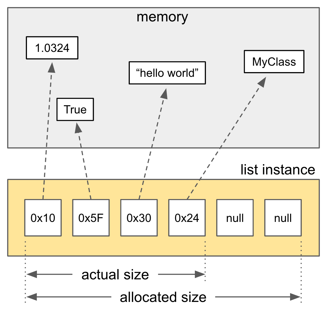
/* Python built-in list */
typedef struct {
    PyObject_VAR_HEAD
    PyObject **ob_item;
    Py_ssize_t allocated;
} PyListObject;

As shown, a list is basically a pointer to pointers (a double pointer). This means even if the elements look adjacent in the list, they might be located in completely different places in memory. That leads to poor cache locality and more cache misses, which can slow things down.

In contrast, Python’s built-in array [2-1] and numpy’s ndarray use a contiguous memory block like a C array. Here’s the structure of Python’s built-in array:

/* Python built-in array */
typedef struct arrayobject {
    PyObject_VAR_HEAD
    char *ob_item;
    Py_ssize_t allocated;
    const struct arraydescr *ob_descr;
    PyObject *weakreflist;
    Py_ssize_t ob_exports;
} arrayobject;

Notice that ob_item is a char* here, not a PyObject** like in lists. So, arrays store the actual values, not references to Python objects. This gives them better memory locality. But the downside is they can only store primitive values like int, float, or byte.

Numpy’s ndarray is implemented in C and also stores values in contiguous memory, making memory access very fast. But if you use dtype='O' in numpy (to store objects), it will behave like a regular Python list, storing references instead of raw values [2-2].

Because of these differences, performance can vary depending on whether you use a list, an array, or an ndarray. Let’s look at two performance comparison examples.

Comparing access performance

You might think that lists are slower due to poor memory locality. But is that really true? Let’s test it:

import timeit
import array
import numpy as np

N = 10000
M = 1000

my_list = [i for i in range(N)]
my_array = array.array('i', my_list)
my_ndarray = np.array(my_list)

def test_list_sum():
    sum(my_list)

def test_array_sum():
    sum(my_array)

def test_numpy_sum():
    sum(my_ndarray)

def test_numpy_npsum():
    np.sum(my_ndarray)

list_time = timeit.timeit(test_list_sum, number=M)
array_time = timeit.timeit(test_array_sum, number=M)
ndarray_sum_time = timeit.timeit(test_numpy_sum, number=M)
ndarray_npsum_time = timeit.timeit(test_numpy_npsum, number=M)

print(f'list: {list_time * 1000:.1f} ms')
print(f'array: {array_time * 1000:.1f} ms')
print(f'ndarray (sum): {ndarray_sum_time * 1000:.1f} ms')
print(f'ndarray (np.sum): {ndarray_npsum_time * 1000:.1f} ms')

Results:

list: 72.0 ms
array: 126.4 ms
ndarray (sum): 373.0 ms
ndarray (np.sum): 2.5 ms

When using np.sum(), numpy is very fast. But with regular sum(), Python’s list is actually faster. Why?

With list, Python reads the value and adds it — simple. But with array or ndarray, the values are primitives, so Python has to convert each one into a Python object before adding. That extra step slows it down.

np.sum() is fast because it’s written in C and operates directly on the primitive values, avoiding conversion overhead. It also uses fast C-level loops and even parallel processing like OpenMP.

So to get the best performance with numpy, avoid using Python for-loops — use vectorized numpy operators instead. If you need to use custom functions, apply_along_axis() [2-3] might help, but it’s still not as fast as pure vectorized operations.

Comparing serialization performance

Another case where performance differs is serialization. When saving arrays to a database or sending them in payloads, you often convert them to binary. Since arrays and ndarrays already store values in binary format, serialization is faster. Lists store scattered references, so it’s much slower.

Let’s use the marshal module to compare the time for serialization and deserialization:

import timeit
import array
import numpy as np
import pickle
import marshal
import random

N = 10000
M = 1000

my_list = [random.random() for _ in range(N)]
my_list_enc = marshal.dumps(my_list)

my_array = array.array('f', my_list)
my_array_enc = marshal.dumps(my_array)

my_ndarray = np.array(my_list, dtype=np.float32)
my_ndarray_enc = marshal.dumps(my_ndarray)

def test_list_marshal():
    marshal.dumps(my_list)

def test_list_unmarshal():
    marshal.loads(my_list_enc)

def test_array_marshal():
    marshal.dumps(my_array)

def test_array_unmarshal():
    marshal.loads(my_array_enc)

def test_ndarray_marshal():
    marshal.dumps(my_ndarray)

def test_ndarray_unmarshal():
    marshal.loads(my_ndarray_enc)

Results:

[marshal]
list: 131.2 ms
array: 0.8 ms
ndarray: 1.9 ms

[unmarshal]
list: 155.4 ms
array: 0.9 ms
ndarray: 0.9 ms

Lists are 80–160 times slower. Even with other serializers like pickle, the results are similar. This is because lists require reading scattered memory and checking the data type of each item.

So even though list, array, and ndarray look similar, their memory structure affects performance. If serialization is a bottleneck, consider using array or ndarray.

Hyperconnect’s Case

At Hyperconnect, we often deal with operations involving vectors made of many floats (like embeddings). We use numpy’s vector operators and fancy indexing to handle large loads efficiently, even for complex logic.

We also saw clear performance improvements in serialization. Our recommendation server reads and writes many vectors to databases. Even when using fast encoders like marshal, deserializing lists caused major overhead. Switching to ndarray cut deserialization time by 80%, improving end-to-end latency.

But as we said before, just using numpy or array doesn’t guarantee better performance. Always test and measure for your specific use case.

#3 Multiprocessing has high communication overhead — be careful in low-latency scenarios

If a CPU operation takes a long time, using parallelism can speed things up. Common approaches include multithreading and multiprocessing. However, as many know, Python’s multithreading is limited due to the Global Interpreter Lock (GIL) [3-1], so it often doesn’t improve performance.

Because of this, the Python community often recommends using multiprocessing instead. But is multiprocessing always the answer? Not necessarily. There are two common problems with Python’s multiprocessing, and you should only use it in environments where these issues don’t occur:

If you don’t create a process pool ahead of time, spawning processes for each request can cause heavy overhead.
Even if you pre-create the pool, if the data shared between processes is large, communication overhead can be significant.

Process spawn overhead

Let’s look at the first problem with an example. The code below calculates fibonacci(25) four times. The /multiprocess endpoint uses a multiprocessing pool to run the function in parallel. The /singleprocess endpoint runs it four times sequentially.

import multiprocessing
import time

from fastapi import FastAPI
app = FastAPI()

def fibonacci(n: int) -> int:
    return n if n <= 1 else fibonacci(n-1) + fibonacci(n-2)

@app.get("/multiprocess")
async def multiprocess_run() -> float:
    start_time = time.time()
    with multiprocessing.Pool(4) as pool:
        pool.map(fibonacci, [25, 25, 25, 25])
    elapsed_time = time.time() - start_time
    print(f"multiprocess elapsed time: {elapsed_time * 1000:.1f}ms")
    return elapsed_time

@app.get("/singleprocess")
async def singleprocess_run() -> float:
    start_time = time.time()
    for _ in range(4):
        fibonacci(25)
    elapsed_time = time.time() - start_time
    print(f"singleprocess elapsed time: {elapsed_time * 1000:.1f}ms")
    return elapsed_time

Results (on macOS):

multiprocess elapsed time: 304.2ms
singleprocess elapsed time: 129.2ms

Surprisingly, the multiprocessing version is more than twice as slow. Why? Because of the overhead from spawning new processes. In Python, processes can be created using either spawn or fork [3-2].

spawn starts a brand new Python interpreter and re-imports everything — slow but safe.
fork copies the current process — faster but less safe if threads are involved [3-2], [3-3].

macOS and Windows use spawn by default, while Unix systems use fork. You can change the method, but each has trade-offs.

So should we avoid both? Not necessarily. The best solution is to avoid spawning processes for each request. Instead, create a process pool at app startup and reuse it.

Here’s the modified example using startup_event_handler:

async def startup_event_handler():
    app.state.process_pool = multiprocessing.Pool(4)

app.add_event_handler("startup", startup_event_handler)

@app.get("/multiprocess")
async def multiprocess_run() -> float:
    start_time = time.time()
    app.state.process_pool.map(fibonacci, [25, 25, 25, 25])
    elapsed_time = time.time() - start_time
    print(f"multiprocess elapsed time: {elapsed_time * 1000:.1f}ms")
    return elapsed_time

Now /multiprocess is much faster:

multiprocess elapsed time: 49.9ms

Communication overhead between processes

So is everything fixed now? Not quite. Let’s look at the second problem: even with a pre-created pool, large data transfers between processes can cause major overhead.

In Python, data sent between processes is serialized using pickle [3-4]. If the data is large, the time spent serializing and deserializing may outweigh the benefit of parallelism.

Here’s an example. We generate 100 vectors of size 512 and sum them element-wise.

/multiprocess: splits data into 4 chunks and processes in parallel.
/singleprocess: sums all vectors in one thread.
A process pool is used to avoid spawn overhead.

import multiprocessing
import random
import time
from typing import List

from fastapi import FastAPI

async def startup_event_handler():
    app.state.process_pool = multiprocessing.Pool(4)

app = FastAPI()
app.add_event_handler("startup", startup_event_handler)

def generate_random_vector(size: int) -> List[float]:
    return [random.random() for _ in range(size)]

def element_wise_sum(vectors: List[List[float]]) -> List[float]:
    ret_vector = [0.0] * len(vectors[0])
    for vector in vectors:
        for i in range(len(vector)):
            ret_vector[i] += vector[i]
    return ret_vector

@app.get("/multiprocess")
async def multiprocess() -> List[float]:
    vectors = [generate_random_vector(512) for _ in range(100)]

    start_time = time.time()
    result_vector_list = app.state.process_pool.map(element_wise_sum, [
        vectors[:25], vectors[25:50], vectors[50:75], vectors[75:],
    ])
    ret_vector = element_wise_sum(result_vector_list)

    elapsed_time = time.time() - start_time
    print(f"multiprocess elapsed time: {elapsed_time * 1000:.1f}ms")
    return ret_vector

@app.get("/singleprocess")
async def singleprocess_run() -> List[float]:
    vectors = [generate_random_vector(512) for _ in range(100)]

    start_time = time.time()
    ret_vector = element_wise_sum(vectors)

    elapsed_time = time.time() - start_time
    print(f"singleprocess elapsed time: {elapsed_time * 1000:.1f}ms")
    return ret_vector

Even though we avoided the spawn overhead, the /multiprocess endpoint is still slower:

multiprocess elapsed time: 12.0ms
singleprocess elapsed time: 10.4ms

This is because the vectors data is large, and sending it between processes creates high communication overhead.

Hyperconnect’s Case

You might think this example is rare, but in ML backends that deal with large datasets, vector computations like this are common. At Hyperconnect, we’ve experienced cases where using multiprocessing actually made things slower due to this overhead — sometimes increasing latency by more than 5%.

So before using Python multiprocessing, make sure you understand the communication patterns in your app. Even when it seems like parallelism would help, we always evaluate the pattern first before deciding whether to implement it.

#4 If you’re using PyTorch in a multiprocess environment, adjust `num_threads`

Pre-forked workers and PyTorch / Numpy conflicts

Backend servers often handle multiple requests at the same time to take advantage of multi-core CPUs. In Python, this is commonly done using pre-forked worker models like gunicorn. At Hyperconnect, we also use gunicorn [4-1] to run multiple pre-forked uvicorn processes (also called Web Workers) in a single pod. This allows us to handle many requests at once and fully use the CPU.

Modern CPUs have multiple cores, so using parallelism usually leads to faster response times and higher throughput. But if your backend app uses PyTorch or Numpy, you need to be careful when running it in a parallel server like gunicorn — it could actually make things slower.

Why? Because PyTorch and Numpy use multithreading for their internal operations (at the C level, not Python’s threading). They try to use all available CPU cores by default. So, if you have a pod with 4 vCPUs and you start 4 web workers, each one will try to use all 4 cores. This leads to CPU contention — workers fight for the same resources, which increases context switching and cache misses, and in the end, reduces performance.

Let’s look at an example

To see this in action, let’s run a simple program that performs a matrix multiplication on 10,000 by 10,000 arrays and check CPU usage using a tool like htop:

import numpy as np
import torch

numpy_a = np.empty(shape=(10000, 10000))
numpy_b = np.empty(shape=(10000, 10000))
numpy_a @ numpy_b

torch_a = torch.from_numpy(numpy_a)
torch_b = torch.from_numpy(numpy_b)
torch_a @ torch_b

Even though we didn’t tell it to use multiple threads, you’ll see that all CPU cores are used during the operation.

cpu usage

By the way, if you see only half the logical cores being used, that’s because the other half are “virtual” cores created by Intel’s Hyper-Threading [4-2]. These virtual cores aren’t as useful for heavy matrix math, so they don’t get used much.

So how do we fix this in a real API server? Here’s a simple FastAPI + PyTorch example:

import os
import time
import multiprocessing as mp
import torch

def foo(i: int) -> None:
    matrix_a = torch.rand(size=(1000, 1000))
    matrix_b = torch.rand(size=(1000, 1000))
    # warm up
    for _ in range(10):
        torch.matmul(matrix_a, matrix_b)

    start_time = time.perf_counter()
    for _ in range(100):
        torch.matmul(matrix_a, matrix_b)
    print(i, time.perf_counter() - start_time)

if __name__ == "__main__":
    num_processes = len(os.sched_getaffinity(0))
    print("num_processes: ", num_processes)
    with mp.Pool(num_processes) as pool:
        pool.map(foo, range(num_processes))

Running this on 4 cores might give results like:

num_processes:  4
process #[1]: 8.69 s
process #[2]: 8.76 s
process #[0]: 8.87 s
process #[3]: 8.80 s

Now let’s limit the number of threads per process to 1 using the OMP_NUM_THREADS environment variable:

OMP_NUM_THREADS=1 taskset 0x55 python main.py

This gives:

num_processes:  4
process #[3]: 1.43 s
process #[2]: 1.43 s
process #[1]: 1.43 s
process #[0]: 1.43 s

That’s 6x faster! Alternatively, if you’re using only PyTorch, you can also use:

torch.set_num_threads(1)

Why do PyTorch and Numpy try to use all CPUs by default? Because they were designed mainly for data analysis and model training — situations where there’s usually one big job and using all resources is the fastest approach [4-3].

Hyperconnect’s Case

At Hyperconnect, we added thread limit settings (1 thread per worker) to FastAPI servers that use PyTorch and to model servers based on Nvidia Triton. In some servers, this change improved both latency and throughput by more than 3x. If you’re using PyTorch with multiple workers, consider trying this — it might be the easiest performance win you can get.

#5 Pydantic is very slow — avoid it when not needed

What is Pydantic?

FastAPI[5-1] is becoming very popular for backend development. It’s a great open-source project — you could even say it’s the better version of Flask. But FastAPI relies on Pydantic[5-2] to define API endpoints. Pydantic helps with data validation (type checking) and parsing. For example:

from datetime import date
from pydantic import BaseModel

class User(BaseModel):
    user_id: int
    birthday: date

User.parse_raw('{"user_id": "100", "birthday": "2000-01-01"}')
# User(user_id=100, datetime.date(2000, 1, 1))

FastAPI deeply integrates with Pydantic — it even uses it to auto-generate Swagger UI. So if you’re using FastAPI, you’re probably using Pydantic too.

Pydantic is very convenient. But don’t overuse it, especially when validation is not needed. Why? Because it’s slow.

How slow is Pydantic?

Let’s compare the time it takes to create 400 Pydantic objects with a float list of length 50:

import timeit
from typing import List
from pydantic import BaseModel

class FeatureSet(BaseModel):
    user_id: int
    features: List[float]

def create_pydantic_instances() -> None:
    for i in range(400):
        obj = FeatureSet(
            user_id=i,
            features=[1.0 * i + j for j in range(50)],
        )

elapsed_time = timeit.timeit(create_pydantic_instances, number=1)
print(f"pydantic: {elapsed_time * 1000:.2f}ms")

Output:

pydantic: 12.29ms

Now let’s do the same thing using a plain Python class:

import timeit
from typing import List

class FeatureSet:
    def __init__(self, user_id: int, features: List[float]) -> None:
        self.user_id = user_id
        self.features = features
    
def create_class_instances() -> None:
    for i in range(400):
        obj = FeatureSet(
            user_id=i,
            features=[1.0 * i + j for j in range(50)],
        )

elapsed_time = timeit.timeit(create_class_instances, number=1)
print(f"class: {elapsed_time * 1000:.2f}ms")

Output:

class: 1.54ms

So Pydantic is about 8x slower than a plain class in this case.

Hyperconnect’s Case

At Hyperconnect, we replaced unnecessary Pydantic usage with vanilla Python classes or built-in dataclass, and saw over 2x latency improvement in our recommendation APIs. In one case, just creating Pydantic objects was taking more than 200ms (p99).

Pydantic is so well known for being slow that version 2 is being rewritten in Rust [5-3]. We’re looking forward to it — but even then, it won’t be faster than plain Python classes. So if you don’t need validation, avoid Pydantic.

Keep reading the aritcle at Part 2.